How TurboQuant Helped Google Cut AI Memory by 6x?

Google Research just introduced TurboQuant. It is a compression algorithm for AI. The numbers behind it are genuinely impressive.

I am not going to call it a deepseek moment, but the project is definitely interesting. With a few core ideas in place, what TurboQuant does becomes obvious. Without those building blocks, it makes no sense at all.

TurboQuant shrinks the KV cache by around 6x with no accuracy loss and no retraining required. That working memory is one of the biggest bottlenecks in long conversations. Making it smaller and faster matters a lot for cost and latency.

How TurboQuant Helped Google Cut AI Memory by 6x? - Building Blocks

First, vectors. When an AI model reads the word king, it does not see letters. It sees a long list of numbers capturing meaning, context, and relationships to other words.

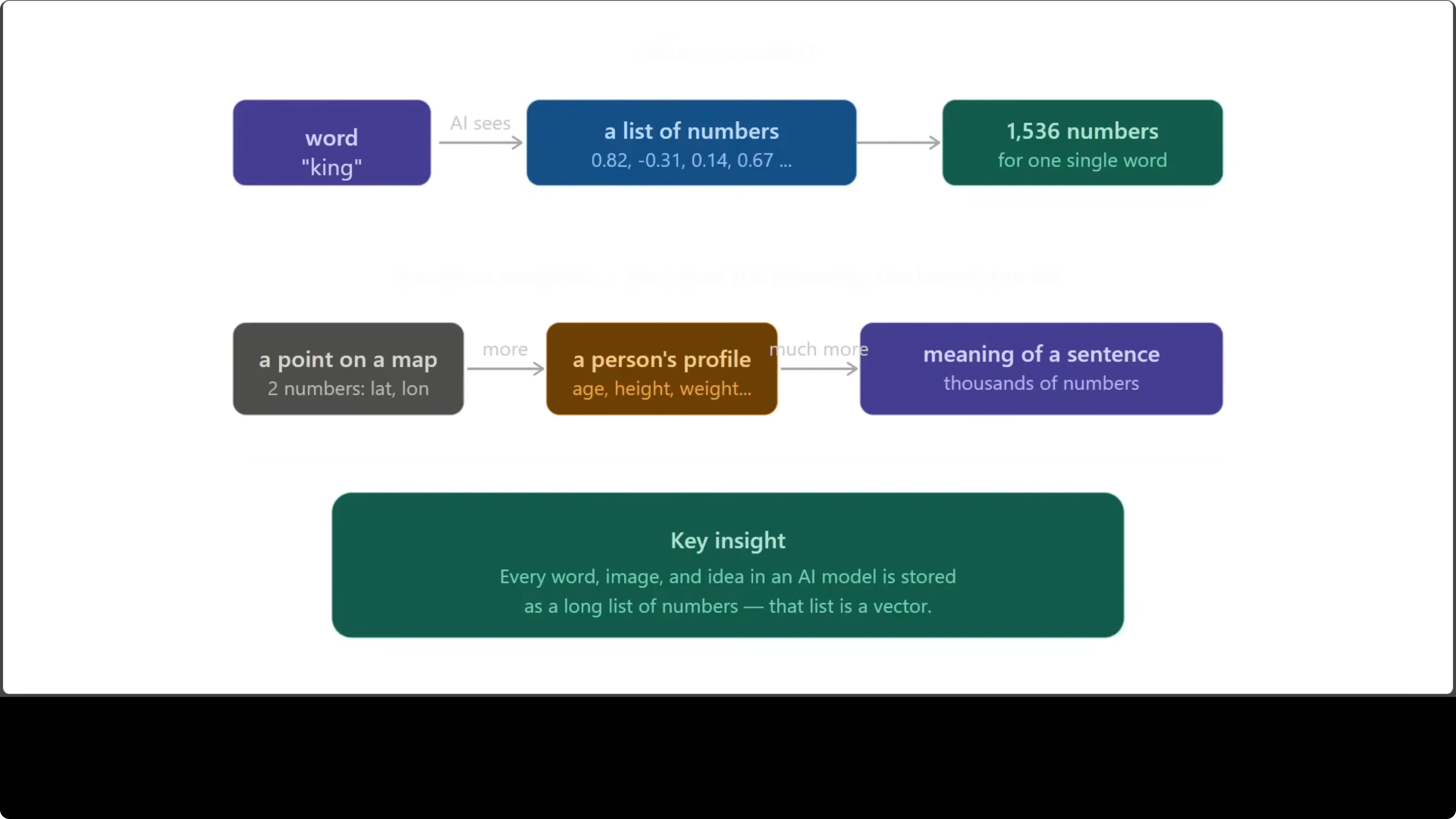
Every single word, sentence, and idea inside a model is stored this way. The richer the concept, the longer the list. A point on a map needs two numbers, while a sentence can need thousands.

Second, quantization. Think of a high resolution photo that still looks the same after light compression. You saved storage and nobody noticed.

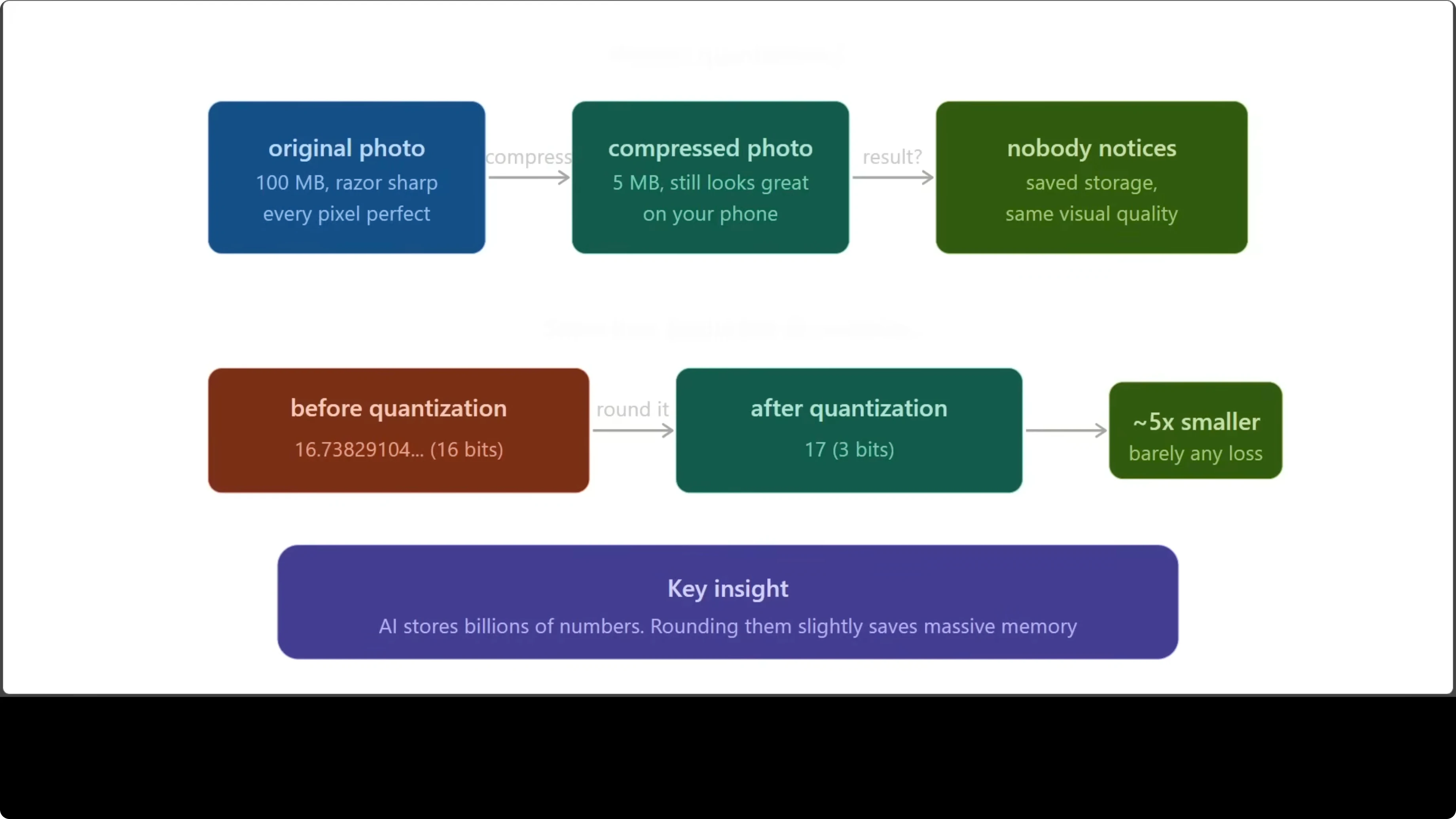
Quantization does the same to numbers. Instead of storing 16.73829104 in 16 bits, you store roughly 17 in a tiny number of bits and keep it close enough. Doing this at scale without hurting quality is the hard part.

Third, the KV cache. It is like a cheat sheet for an open book exam. Fast to read and full of the important bits while a conversation unfolds.

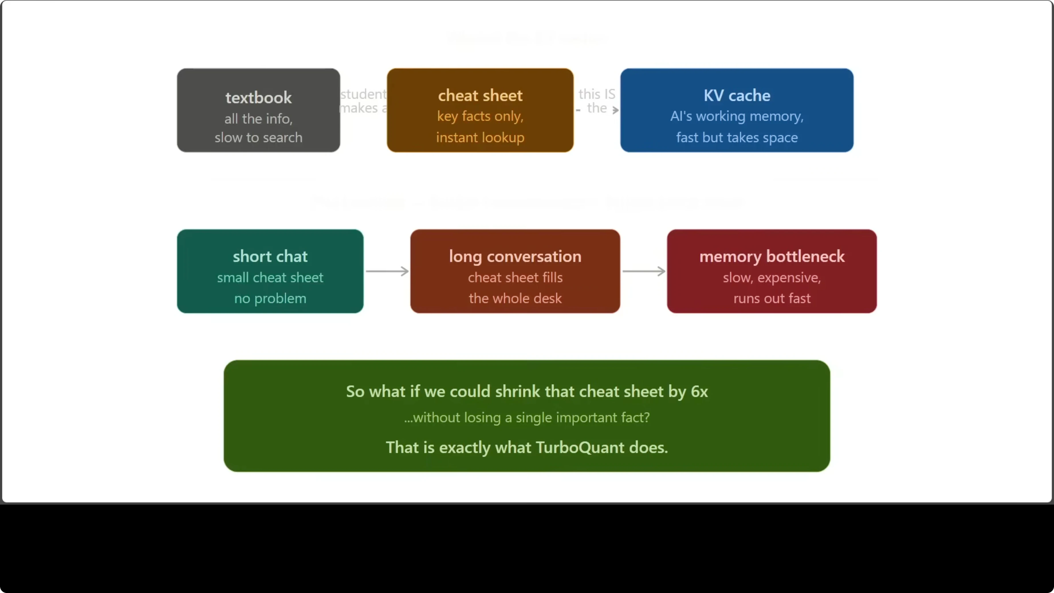
As context grows to thousands or millions of tokens, that cache balloons. It becomes expensive and slow. This is the bottleneck TurboQuant targets.

Read a plain-English explainer on TurboQuant and why the 6x figure matters.

How TurboQuant Helped Google Cut AI Memory by 6x? - The Two Tricks

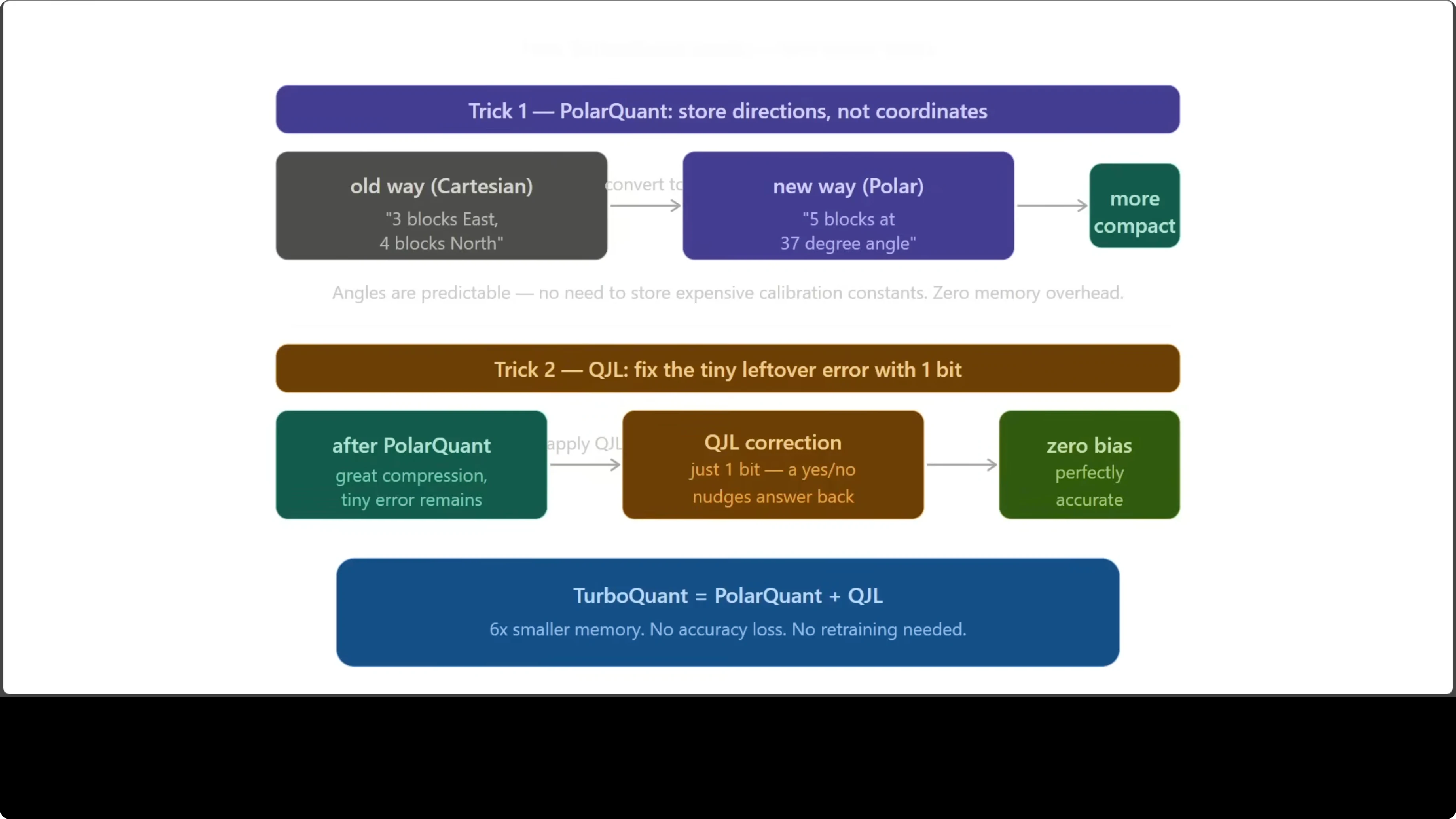
There are two main tricks at play. The first is a polar transform based compression step. The second is a 1-bit correction technique called QJL.

Polar compression converts vectors from standard Cartesian coordinates to a compact angle-radius form. Think of replacing go 3 blocks east and 4 blocks north with go 5 blocks at a 37 degree angle. Same destination, but the angle based description is more predictable and more compact.

The key detail is calibration. Polar style methods remove overhead that traditional schemes need for storing calibration constants. That overhead is eliminated.

Polar transform in code

import numpy as np

def cartesian_to_polar(xy: np.ndarray):
    # xy: shape [N, 2]
    x, y = xy[:, 0], xy[:, 1]
    r = np.sqrt(x * x + y * y)
    theta = np.arctan2(y, x)  # angle in radians
    return r, theta

def quantize_uniform(values: np.ndarray, bits: int, vmin: float, vmax: float):
    # Map continuous values into 2**bits bins in [vmin, vmax]
    levels = 1 << bits
    clipped = np.clip(values, vmin, vmax)
    scale = (levels - 1) / (vmax - vmin + 1e-12)
    q = np.round((clipped - vmin) * scale).astype(np.int32)
    deq = q / scale + vmin
    return q, deq

# Example: compress 2D keys with a polar transform
keys = np.random.randn(1000, 2).astype(np.float32)
r, theta = cartesian_to_polar(keys)

# Quantize radius and angle to a few bits
qr, r_hat = quantize_uniform(r, bits=8, vmin=0.0, vmax=5.0)
qt, t_hat = quantize_uniform(theta, bits=8, vmin=-np.pi, vmax=np.pi)

# Reconstruct approximate keys from quantized polar
x_hat = r_hat * np.cos(t_hat)
y_hat = r_hat * np.sin(t_hat)
reconstructed = np.stack([x_hat, y_hat], axis=1)

In higher dimensions, a generalization of this idea creates a compact representation with predictable structure. That predictable structure is what makes it efficient for KV cache storage.

QJL 1-bit correction

After polar compression, there is a small residual error like being two steps off your destination. QJL uses a single bit per number to nudge the answer back to the right place. One bit, zero bias, and the result is mathematically clean.

QJL stands for Quantized Johnson-Lindenstrauss. The Johnson-Lindenstrauss theorem from the 1980s says you can project high dimensional data into a lower dimensional space while preserving pairwise distances. Here, that transform is paired with 1-bit quantization to capture the sign information needed to correct residuals.

A tiny QJL toy example

import numpy as np

def jl_project(x: np.ndarray, proj: np.ndarray):
    # x: [D], proj: [d, D], returns [d]
    return proj @ x

def one_bit_quantize(z: np.ndarray):
    # Store only the sign bit of each projected component
    return (z >= 0).astype(np.int8)  # 1 for positive, 0 for negative

def one_bit_dequantize(bits: np.ndarray, scale: float):
    # Reconstruct signs and apply a shared scale for magnitude
    signs = np.where(bits > 0, 1.0, -1.0)
    return signs * scale

# Build a random JL matrix
D, d = 1024, 128
proj = np.random.randn(d, D).astype(np.float32) / np.sqrt(d)

x = np.random.randn(D).astype(np.float32)
z = jl_project(x, proj)

# Keep only one bit per entry
bits = one_bit_quantize(z)

# A global scale can be estimated per block to control error
scale = np.mean(np.abs(z)) + 1e-6
z_hat = one_bit_dequantize(bits, scale)

TurboQuant combines the polar style compression with QJL based 1-bit correction. The outcome is a KV cache that is far smaller yet faithful to the original. No retraining is needed.

How TurboQuant Helped Google Cut AI Memory by 6x? - Results

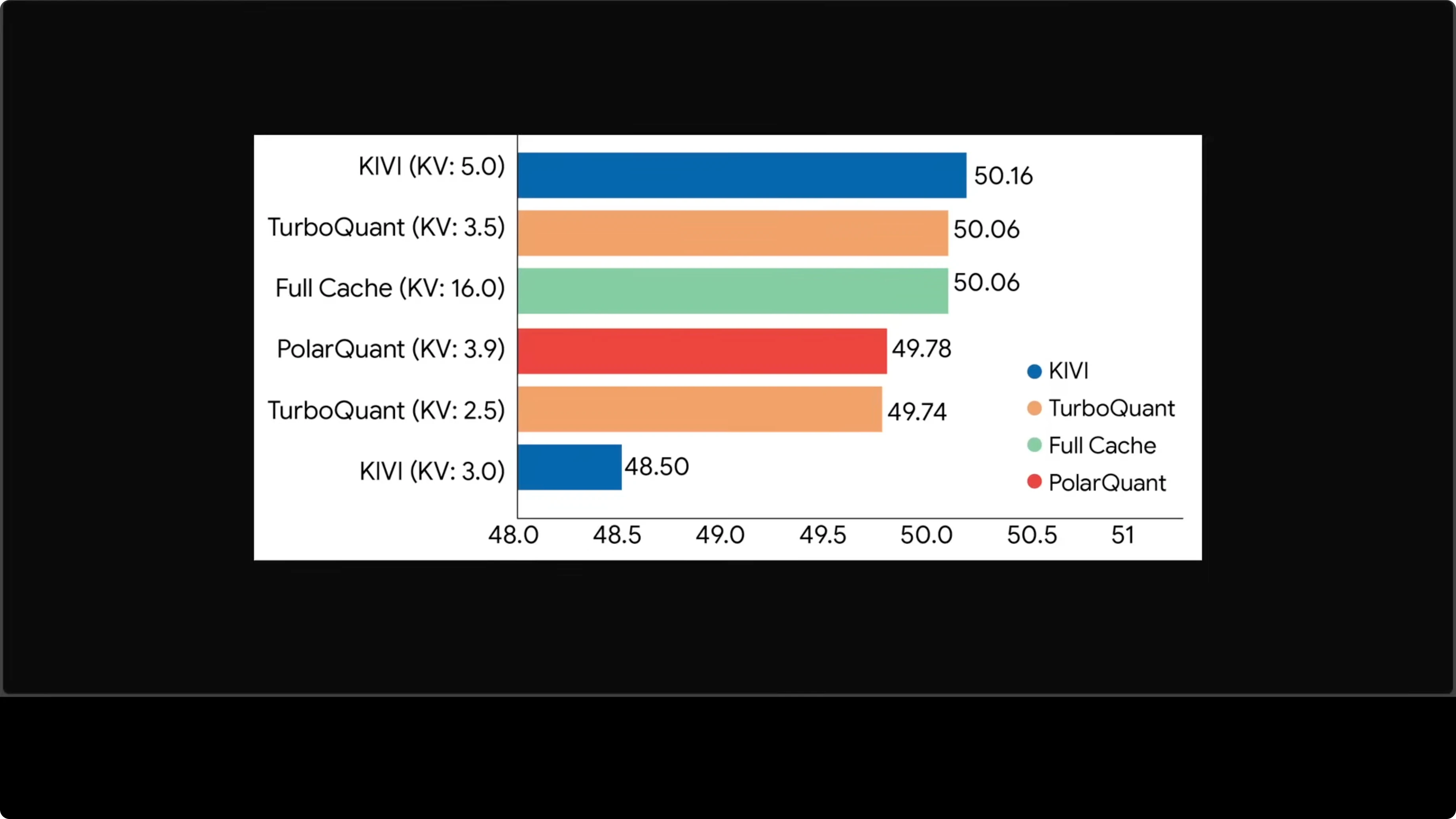
On real tasks like question answering, coding, and summarization, TurboQuant at roughly 3.5 bits matches a full cache at 16 bits. That is a strong result given the compression rate. The accuracy holds while memory drops.

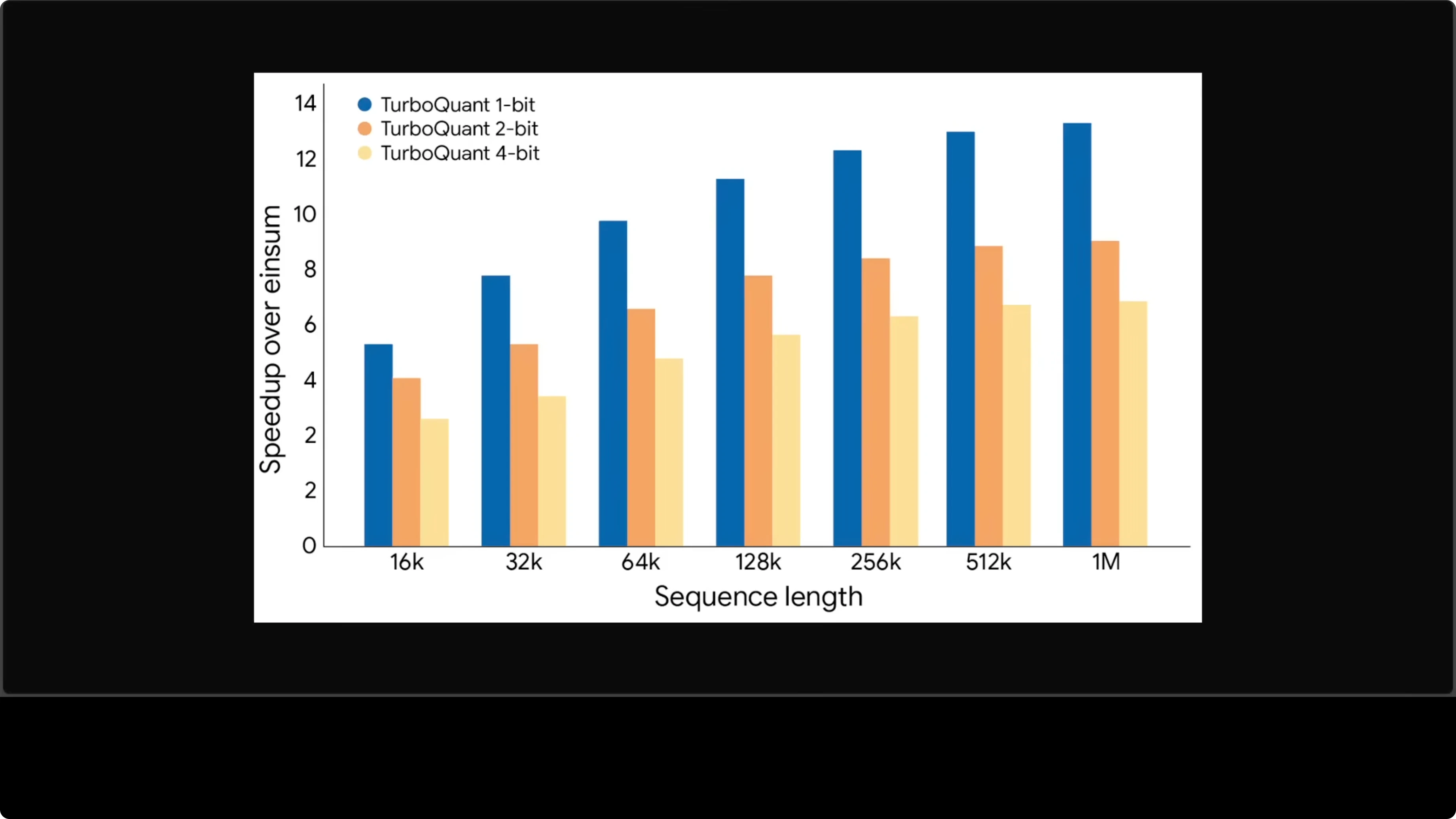
At a million tokens of context, attention computation is up to 13x faster than the uncompressed baseline. The longer the context, the bigger the advantage. That speedup directly translates into lower latency and lower cost.

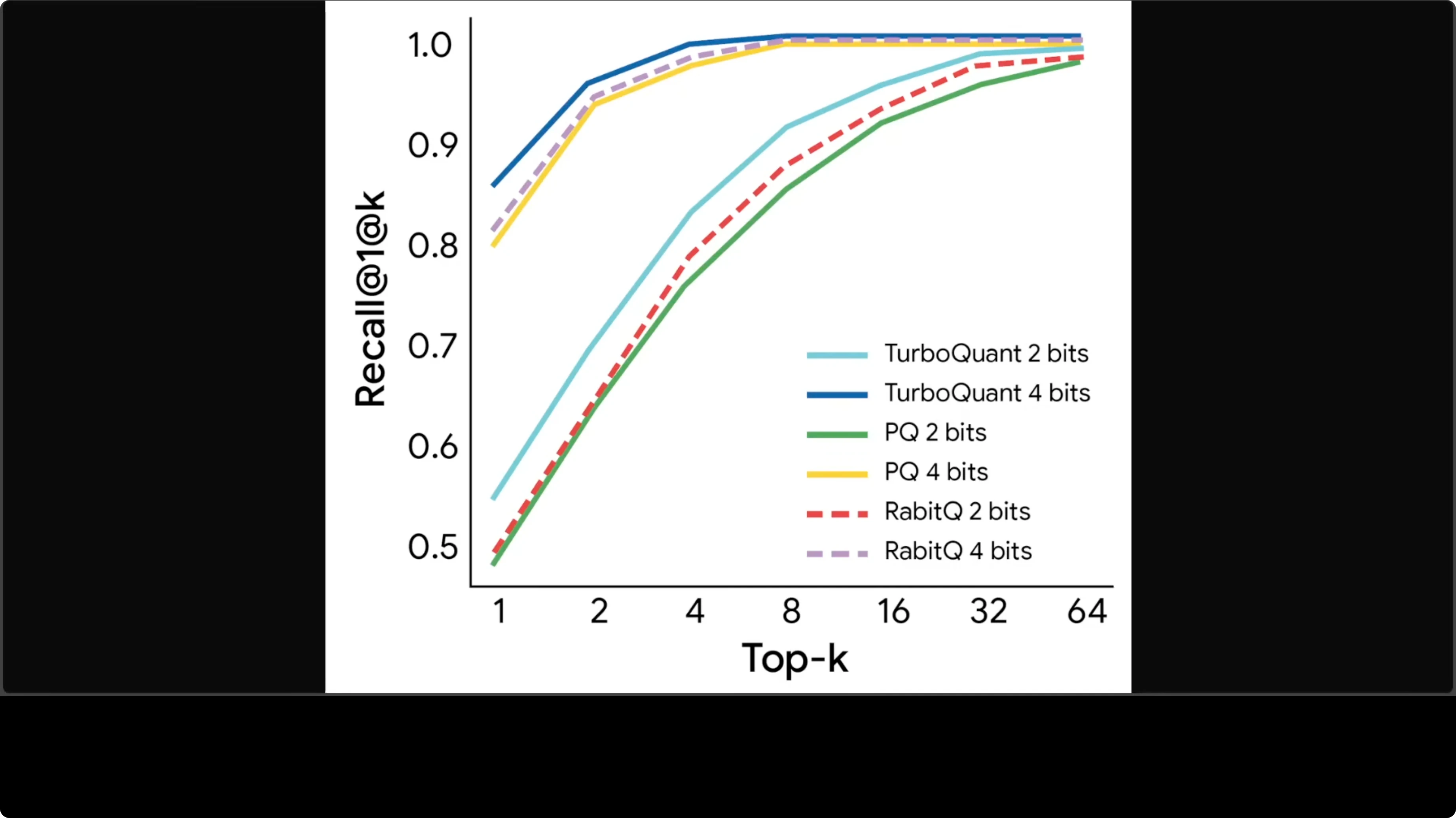
Vector search recall is also strong. The 4-bit line for TurboQuant sits above competitors at every value of K. Better compression and better recall without trade-offs is rare.

Read More: See how quota planning impacts long-context experiments.

How TurboQuant Helped Google Cut AI Memory by 6x? - Quick Start

Identify the KV cache tensors for keys and values in your model. Confirm their shapes across layers and heads.

Apply a polar style transform to convert each block of Cartesian coordinates into a compact angle-radius representation. Quantize those components to the target bit width.

Project residuals through a Johnson-Lindenstrauss matrix. Quantize the signs to one bit per component and store a small scale per block.

During decoding, reconstruct polar components, invert back to Cartesian, and apply the 1-bit sign corrections. Feed the reconstructed KV tensors into attention as usual.

Validate on a held-out set to confirm no loss in perplexity or task scores. Profile memory, speed, and cost across context lengths.

Minimal pseudo-API

def encode_kv_cache(K, V, config):
    # K, V: [layers, heads, seq, dim]
    Kp = polar_encode(K, config.polar_bits)
    Vp = polar_encode(V, config.polar_bits)
    Kcorr = qjl_signs(K - polar_decode(Kp), config.jl_matrix, config.scale_policy)
    Vcorr = qjl_signs(V - polar_decode(Vp), config.jl_matrix, config.scale_policy)
    return PackedKV(Kp, Vp, Kcorr, Vcorr)

def decode_kv_cache(packed, config):
    K = polar_decode(packed.Kp)
    V = polar_decode(packed.Vp)
    K += qjl_reconstruct(packed.Kcorr, config.jl_matrix, config.scale_policy)
    V += qjl_reconstruct(packed.Vcorr, config.jl_matrix, config.scale_policy)
    return K, V

How TurboQuant Helped Google Cut AI Memory by 6x? - Use Cases

Long-form chat agents benefit immediately. KV cache memory shrinks by around 6x, so serving costs drop and throughput rises. That means more concurrent users for the same hardware.

Vector search pipelines that re-rank with attention can hold longer contexts. Better recall at the same memory budget helps retrieval quality. Coding assistants and summarizers also see gains in speed at high token counts.

On-device or edge inference can fit larger context windows. Memory is the limiting factor there, and this is exactly what TurboQuant minimizes. The lack of retraining keeps integration simple.

If you are testing this inside Google AI Studio and run into permission issues, see these quick fixes. Fix common Permission Denied errors in Studio and address Failed to Generate Content due to permissions.

Teams experimenting with restricted accounts may also hit access blocks. For context on account level limits and how they get enforced in practice, see this note on account restrictions. Clear access reduces noise when benchmarking compression.

How TurboQuant Helped Google Cut AI Memory by 6x? - Status and Outlook

TurboQuant is still a research paper. It has not shipped in production yet, though many variants are already being tried. I am holding my horses until a maintained library or official release lands.

I expect details to change when it becomes a product. If it holds up, most large models will run longer conversations at lower cost and higher speed. Search and retrieval systems that lean on vectors will see a direct benefit at scale.

There are many quantization techniques out there already, including RQ, PQ, SpinQuant, GSA, and others. TurboQuant earns attention because it shows strong accuracy at very low bit rates. That combination is rare in practice.

Final Thoughts

TurboQuant targets the KV cache bottleneck with a smart pairing of polar compression and QJL 1-bit correction. The measured gains show around 6x memory savings and large speedups at long context.

No retraining and clean accuracy make adoption attractive. If the research results translate to production, responses will get faster, cheaper, and more accurate at scale.