

How Google’s TIPSv2 Outperforms Competitors Locally?
What if one AI model could tell you what is in an image, where it is, and match it to text all at once. That is exactly what Google DeepMind’s TIPSv2 does. One model, zero shot classification, segmentation, depth estimation, no fine tuning.
I am running it locally on Ubuntu. The system has a single Nvidia RTX A6000 with 48 GB VRAM, though the model also runs on CPU. The checkpoint is small at about 784 MB, which makes local work straightforward.
Why TIPSv2 outperforms competitors locally
Most image AI models are good at one thing. CLIP can match images to text but has no idea about spatial layout. DINOv2 understands spatial detail well but cannot process text at all.TIPSv2 combines both worlds. It brings global understanding, spatial understanding, and text alignment into one shared space. That is the key that lets it handle multiple tasks without task specific training.
For more Google focused research roundups and tools, see the Google collection. You can also explore practical build guides inside Google AI Studio resources if you work across local and cloud workflows.
Architecture overview
TIPSv2 has two encoders, an image encoder and a text encoder. You feed it an image and a text description, and both are converted into embeddings that live in the same shared space. Because the image encoder is spatially aware, those embeddings carry where things are, not just what things are.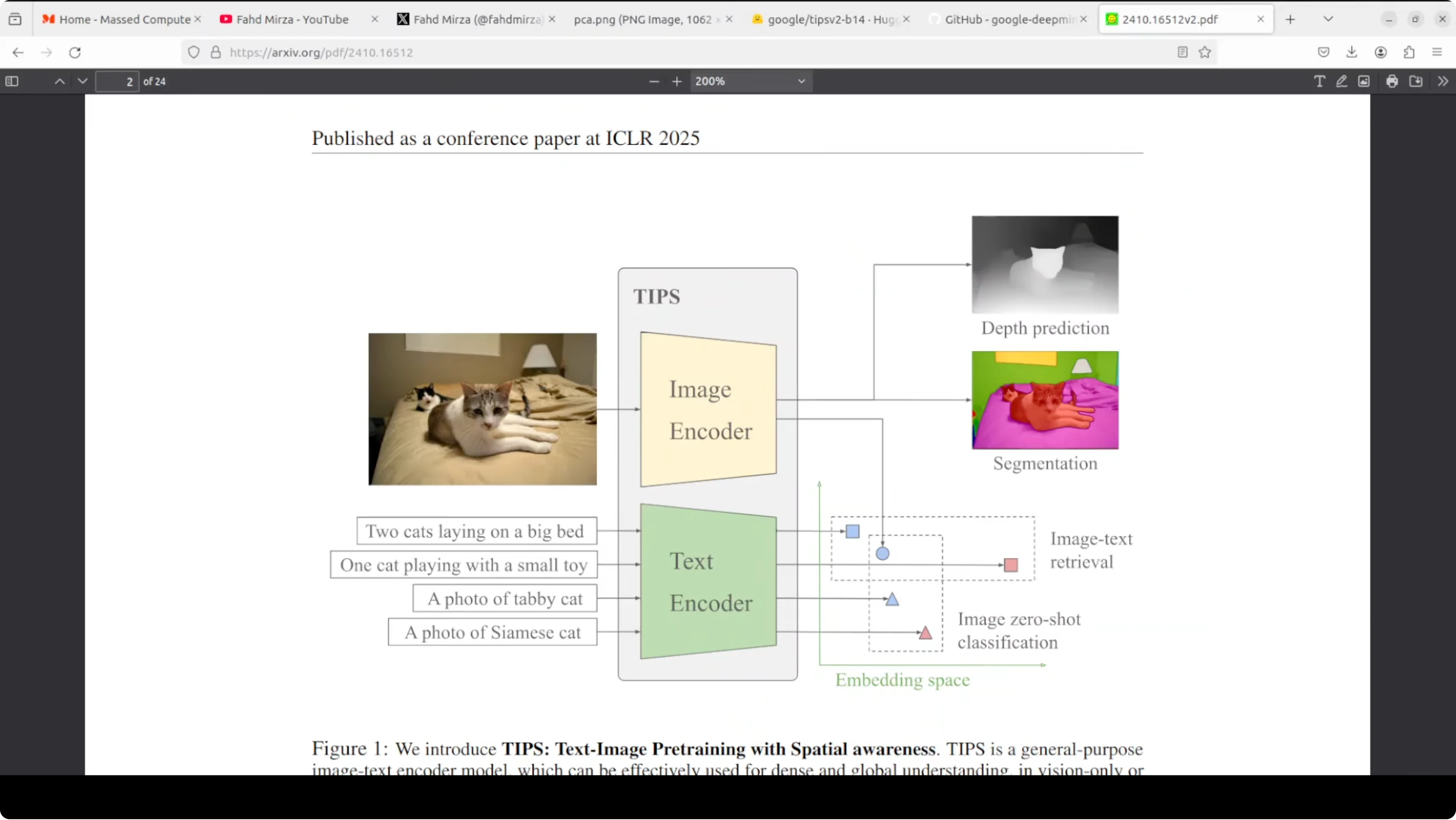
Shared space for text and image
You can do zero shot classification with no training. Ask it to match an image against a set of labels, and the closest text embedding wins. The same shared space enables image text retrieval in either direction.Spatial tokens make the difference
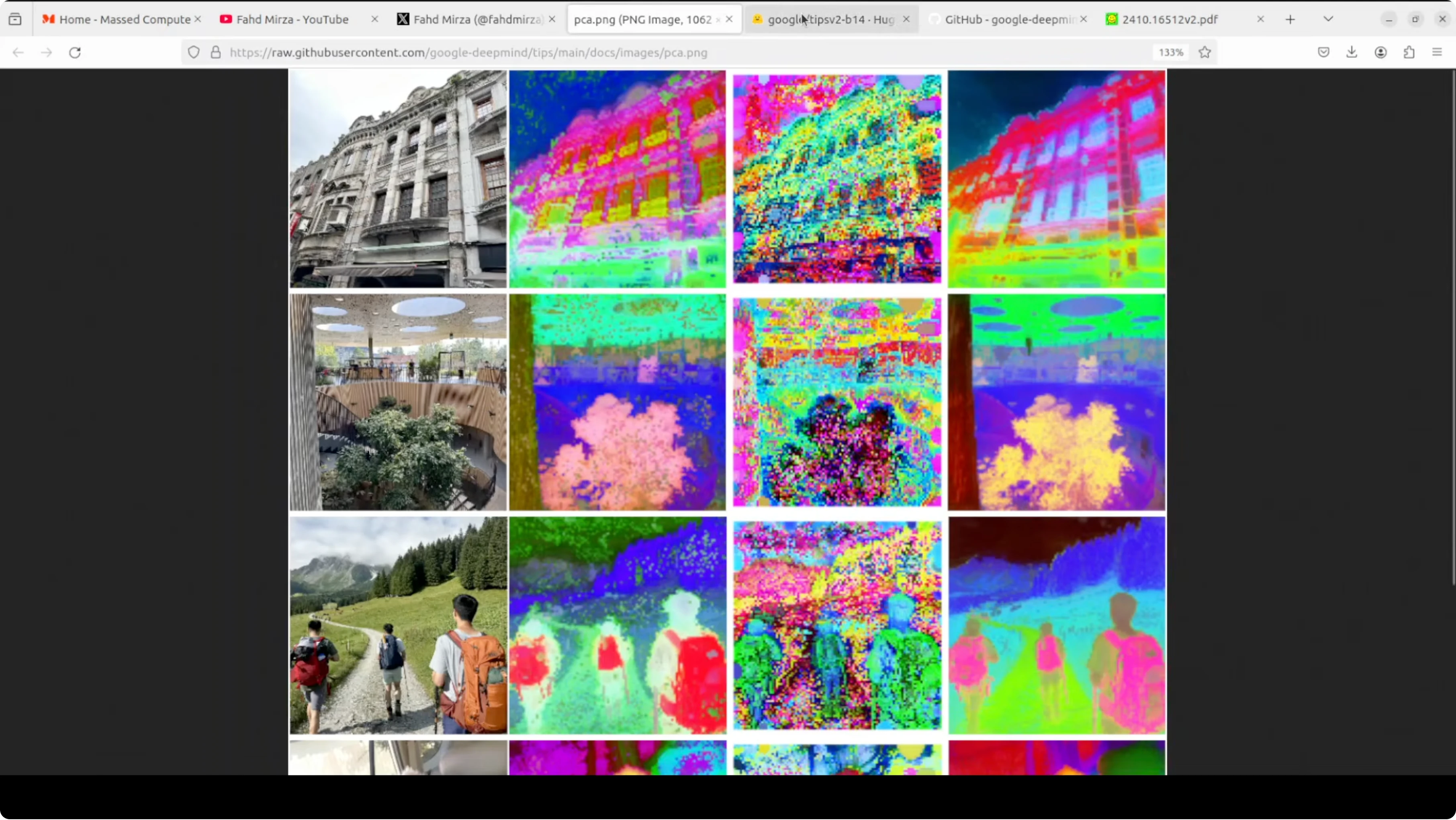
The image encoder outputs a global classification token that summarizes the image. It also outputs patch tokens, one per spatial patch, which capture local detail and position. This spatial awareness is what makes segmentation and depth prediction possible with the same backbone.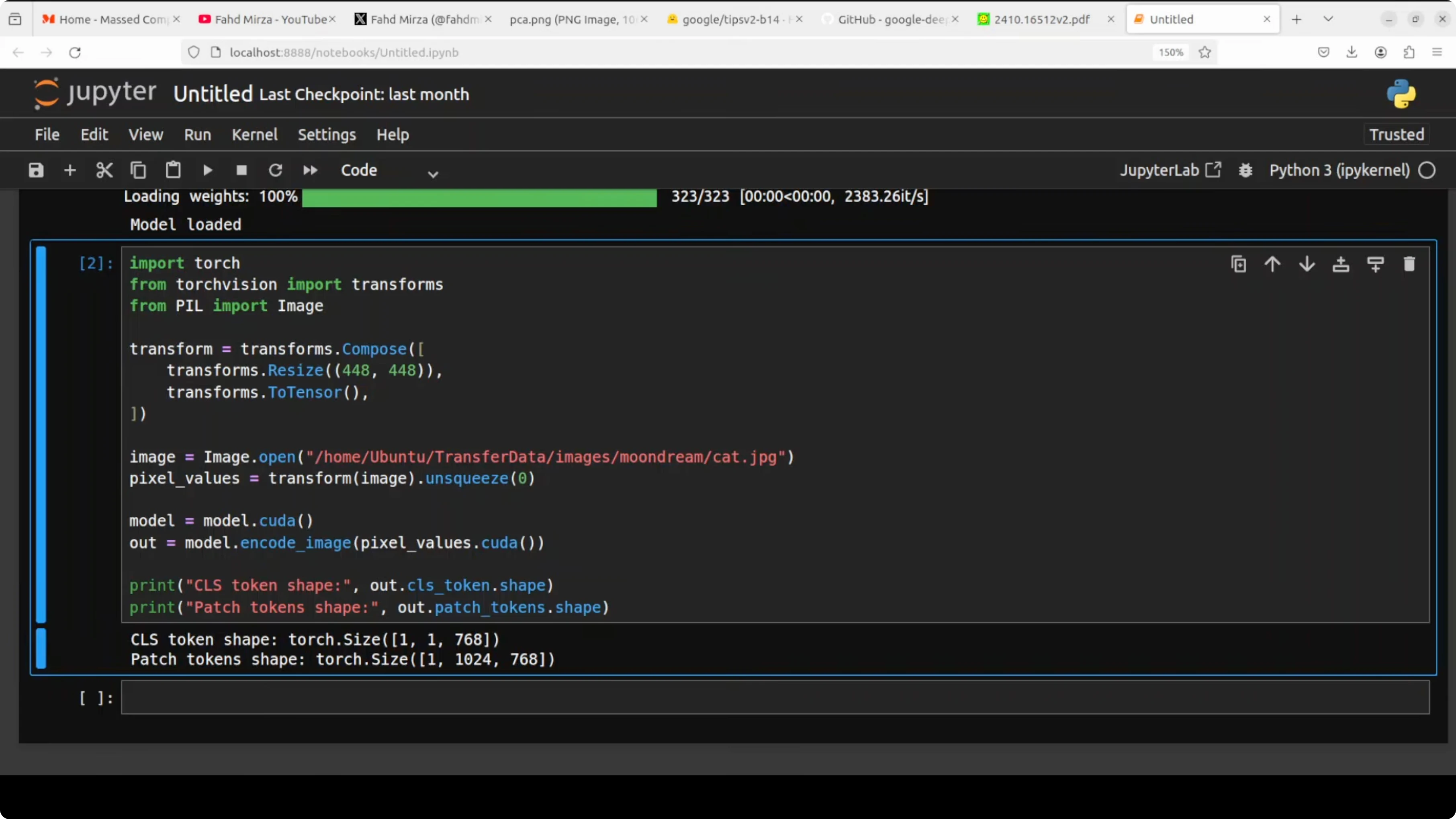
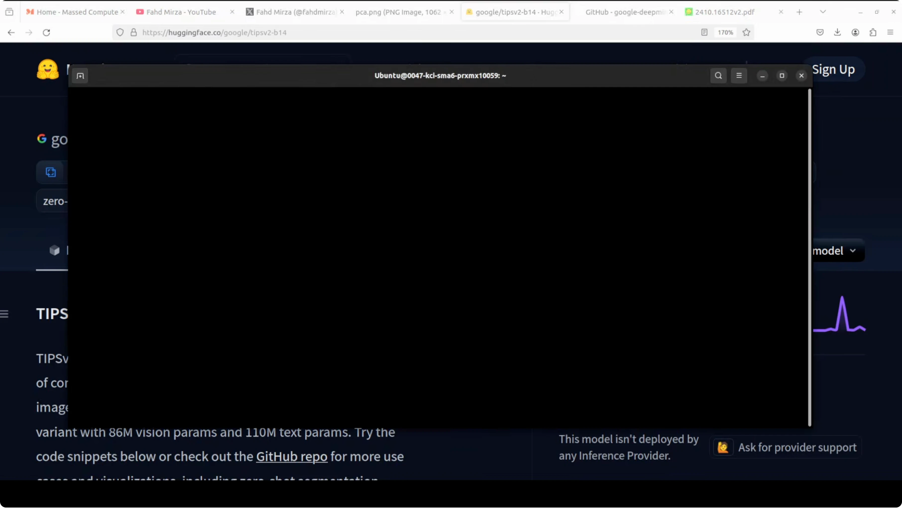
Local setup on Ubuntu
I used a Python virtual environment and Jupyter to run quick tests. The model size and memory footprint keep VRAM use near the 1 GB mark during inference. You can run it on CPU if a GPU is not available, just with slower throughput.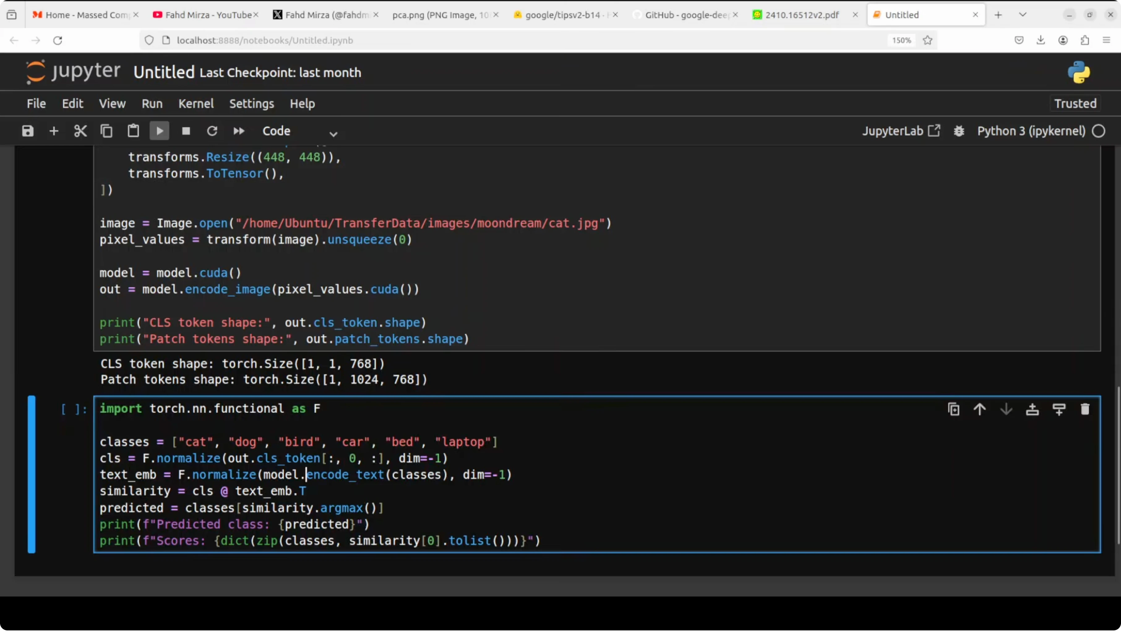
Create the environment
Run these commands in a terminal.python3 -m venv .venv
source .venv/bin/activate
python -m pip install --upgrade pipInstall dependencies
Install PyTorch and basic tooling. Replace cu121 with the CUDA version on your machine or switch to cpu wheels.# GPU wheels
pip install torch torchvision --index-url https://download.pytorch.org/whl/cu121
# Common Python packages
pip install jupyter numpy pillow scikit-learn matplotlib requests tqdmLaunch Jupyter
Start a notebook to keep experiments tidy.jupyter notebookIf you are exploring local fine tuning flows side by side, see our guide on running medium sized models at home in this Qwen local fine tune walkthrough. It pairs well with a TIPSv2 style encoder for quick downstream trials.
Load the model and run inference
The following template shows a clean pattern for working with a dual encoder. Replace the checkpoint path and import lines with the actual TIPSv2 package or repo you use.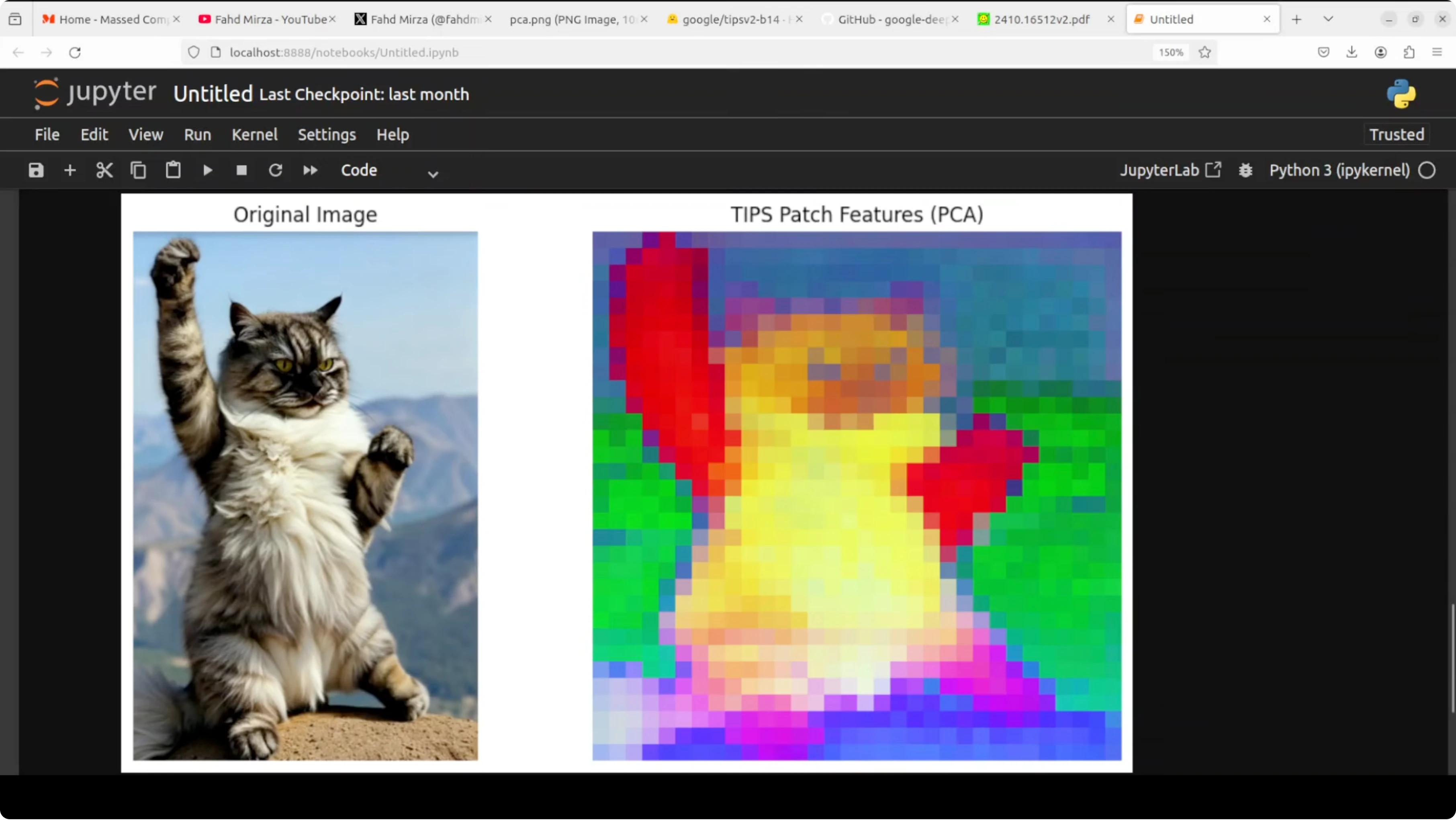
import torch
import torch.nn.functional as F
from PIL import Image
from torchvision import transforms

device = torch.device("cuda" if torch.cuda.is_available() else "cpu")

# Replace these stubs with the real TIPSv2 model loader
class TIPSv2:
    def __init__(self, image_encoder, text_encoder, processor):
        self.image_encoder = image_encoder.to(device).eval()
        self.text_encoder = text_encoder.to(device).eval()
        self.processor = processor

    @torch.inference_mode()
    def encode_image(self, image):
        x = self.processor(image).to(device)
        # Returns a dict with 'cls' and 'patches'
        return self.image_encoder(x)

    @torch.inference_mode()
    def encode_text(self, texts):
        # Returns a tensor of shape [N, D]
        return self.text_encoder(texts)

# Example processor that resizes to 448 and normalizes
def build_image_processor(img_size=448):
    return transforms.Compose([
        transforms.Resize((img_size, img_size), interpolation=transforms.InterpolationMode.BICUBIC),
        transforms.ToTensor(),
        transforms.Normalize(mean=[0.48145466, 0.4578275, 0.40821073],
                             std=[0.26862954, 0.26130258, 0.27577711]),
        lambda x: x.unsqueeze(0)
    ])

# TODO: plug in the real encoders from the official release
image_encoder = ...  # e.g., load_image_encoder(checkpoint_path)
text_encoder  = ...  # e.g., load_text_encoder(checkpoint_path)
processor     = build_image_processor()

tips = TIPSv2(image_encoder, text_encoder, processor)
Global and patch embeddings
Feed an image to the image encoder and inspect both the global summary and the patch level tokens.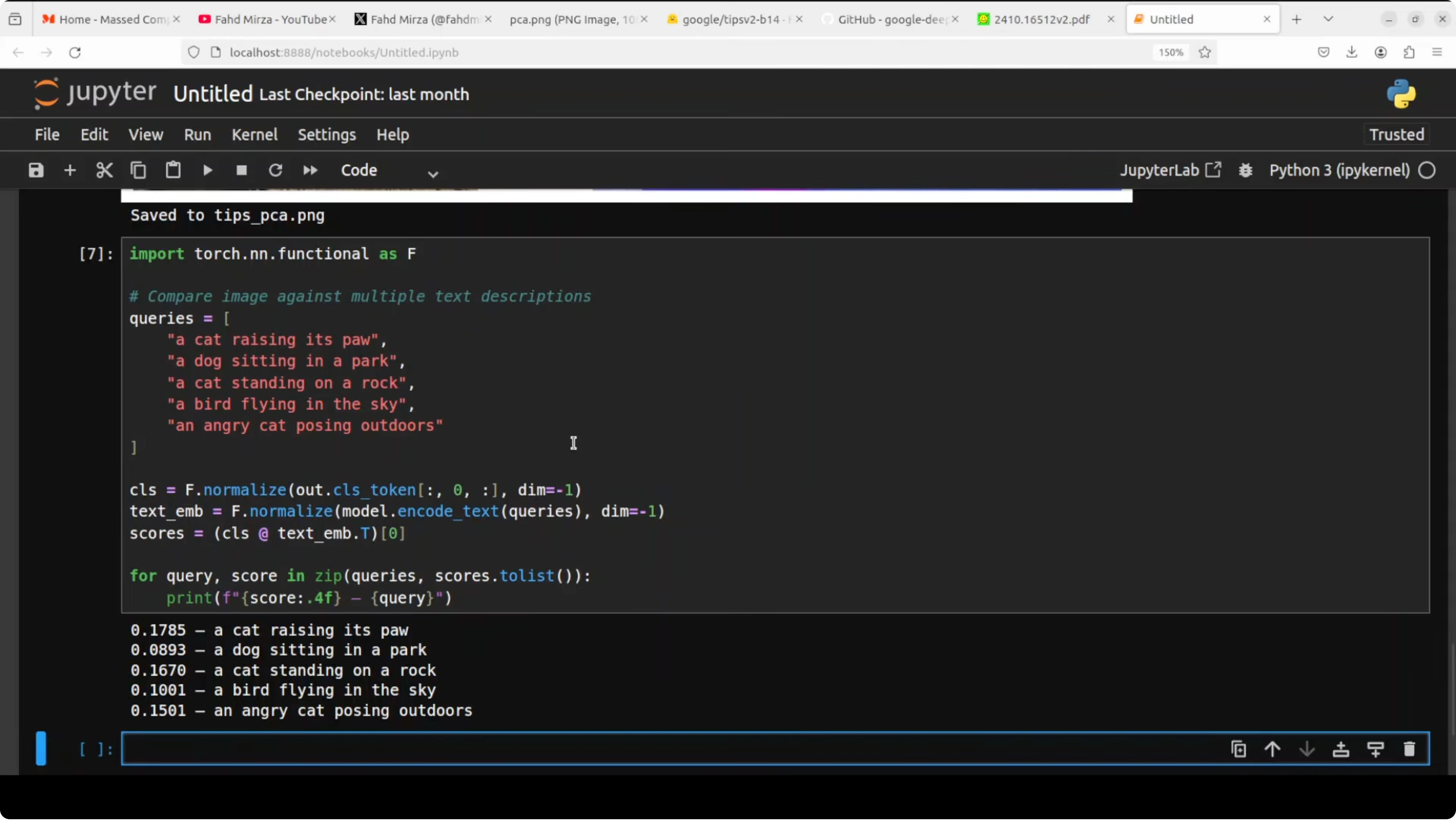
from pathlib import Path

img_path = Path("path_to_your_image.jpg")
image = Image.open(img_path).convert("RGB")

with torch.inference_mode():
    out = tips.encode_image(image)

# Expected keys: 'cls' -> [1, D], 'patches' -> [1, N, D]
cls = out["cls"]           # shape [1, 768] for a base model
patches = out["patches"]   # shape [1, 1024, 768] for a 32x32 grid

print("CLS shape:", tuple(cls.shape))
print("Patches shape:", tuple(patches.shape))
The classification token is a single vector that summarizes the entire image. Patch tokens represent small regions and their spatial context. Together they carry what and where in one pass.
Zero shot classification
Pass a set of text labels, get the closest match to the image embedding with cosine similarity.def l2_normalize(x, dim=-1, eps=1e-12):
return x / (x.norm(dim=dim, keepdim=True) + eps)
def cosine_sim(a, b):
return a @ b.t()
labels = [
"cat",
"dog",
"bird",
"a cat standing on rocky ground outdoors",
"a paw raised"
]
with torch.inference_mode():
img_vec = l2_normalize(cls, dim=-1) # [1, D]
txt_vec = l2_normalize(tips.encode_text(labels), -1) # [L, D]
sims = cosine_sim(img_vec, txt_vec).squeeze(0) # [L]
topk = torch.topk(sims, k=min(5, len(labels)))
for idx in topk.indices.tolist():
print(labels[idx], float(sims[idx]))Image text retrieval
Encode multiple captions and rank them by similarity to the same image embedding.queries = [
"a close up of a pet on a rock",
"an animal outdoors",
"a person riding a bike",
"a scenic mountain view",
"a raised paw"
]
with torch.inference_mode():
q_vec = l2_normalize(tips.encode_text(queries), -1) # [Q, D]
scores = cosine_sim(img_vec, q_vec).squeeze(0) # [Q]
order = torch.argsort(scores, descending=True).tolist()
for i in order:
print(queries[i], float(scores[i]))When moving between local experiments and Google tools, account and quota controls can interrupt workflow. If you ever hit restrictions while testing prompts or models, see this fix for the account restricted issue to get unblocked quickly.
Performance notes
The checkpoint is under 1 GB and the VRAM footprint during inference sits around the 1 GB mark in my tests. You can run the same code on CPU if a GPU is not present. The model remains responsive for quick local iteration.Use cases
Zero shot tagging for large photo libraries without labeled data. Promptable segmentation masks for creative tools and pre annotation in labeling pipelines. Depth cues for robotics, AR prototyping, and 3D aware effects.Image text search in local archives with natural phrases. Rapid visual QA over screenshots and design boards using text prompts. One encoder stack makes these tasks consistent to maintain and scale.
If your workflow also touches Google AI Studio for prompt testing, this guide can help resolve permission denied errors during content generation. For broader coverage of tools and updates in that suite, explore the Google AI Studio category as well.
Final thoughts
TIPSv2 stands out because one model handles global meaning, spatial detail, and text alignment together. That unified design supports zero shot classification, segmentation signals, depth cues, and retrieval without fine tuning. Google DeepMind’s direction here makes local experiments practical and fast, with bigger variants available for those who need extra capacity.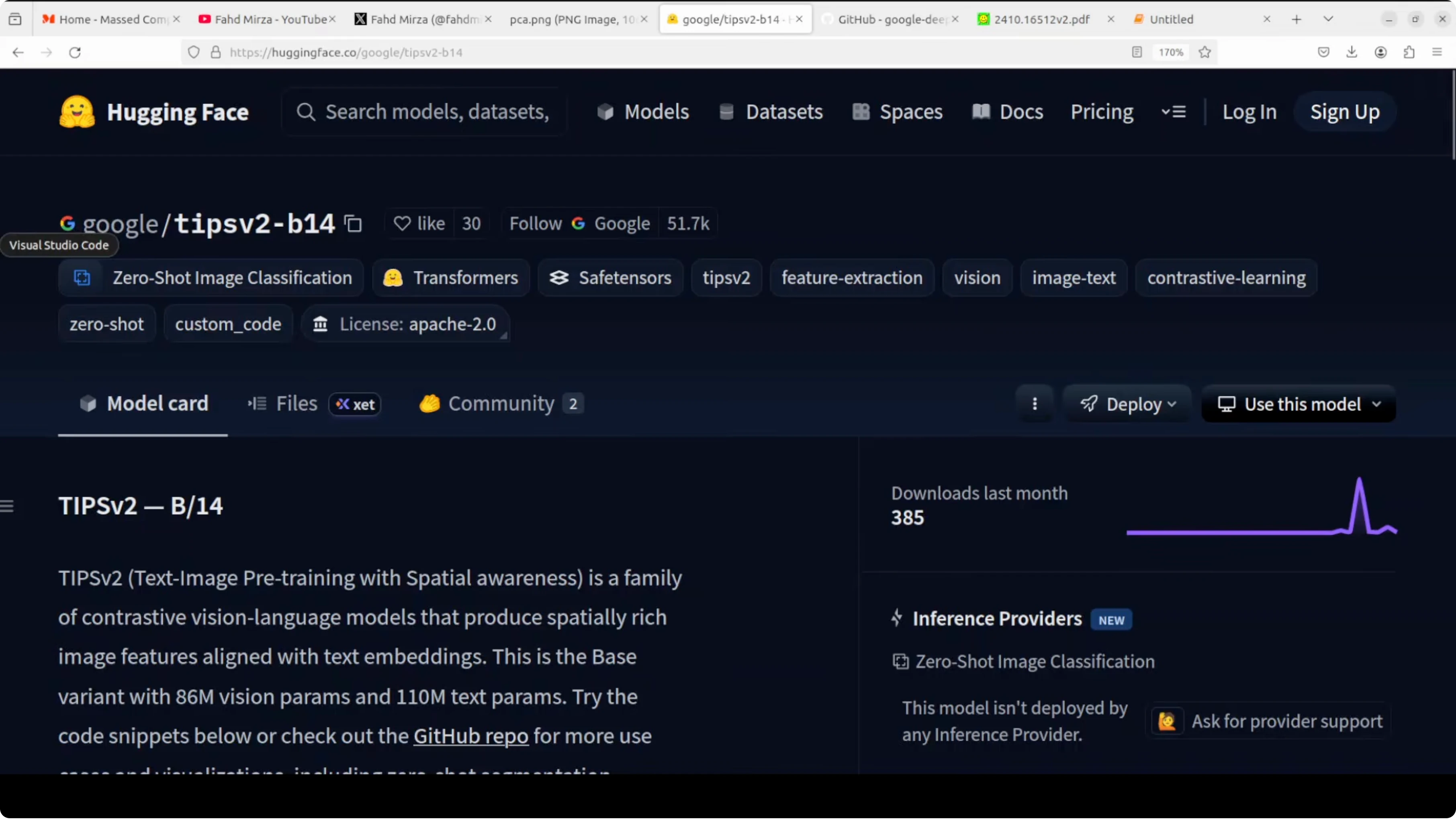
For more company news and releases around this space, browse related notes in our Google hub. If you mix local experimentation and fine tuning in your stack, the local fine tuning tutorial pairs well with an encoder like this for complete workflows.
Subscribe to our newsletter
Get the latest updates and articles directly in your inbox.

Related Posts

8 Best Claude Code Plugins in 2026 (You Need to Know)
8 Best Claude Code Plugins in 2026 (You Need to Know)

7 Best Claude Code Skills (You Need to Know)
7 Best Claude Code Skills (You Need to Know)

Claude Code Desktop IDE Features (You Need to Know)
Claude Code Desktop IDE Features (You Need to Know)